Using Excel 2010 - Manipulating Data

Calculations can easily be set-up in Excel and it is particularly useful to do this when dealing with repetitive calculations. The reasons for doing so are twofold:

• Overall it should work out to be less time consuming than performing them by hand.
• If a mistake in the calculation is made, correcting the error in the affected spreadsheet cell(s) will automatically result in all the calculations being updated; rather than having to repeat all the (by hand) calculations.

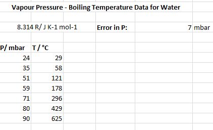
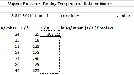
1.	On a new sheet (e.g. Sheet3) in your workbook, enter the data given below, so that it looks like the figure shown.
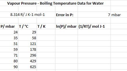
2.	Rather than plotting P vs T, we wish to linearise the data, so that the plot will be a straight line. Using the integrated form of the Clausius-Clapeyron equation it can be shown that a plot of ln(P) vs 1/RT will be linear. So we need to calculate ln(P) and 1/RT for each of the data points. To do this we first label the columns where this transformed data will appear. Edit your spreadsheet until it appears like the figure opposite.
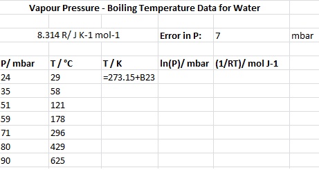
3.	To calculate the first value in the T / K column, select cell C6 and then type =b6+273.15 Note 1: The = at the start of the entry specifies you are typing a formula, i.e. that you wish to calculate a value. Note 2: Entering b6 causes Excel to use the value it finds in cell B6 when it calculates the value of the formula.
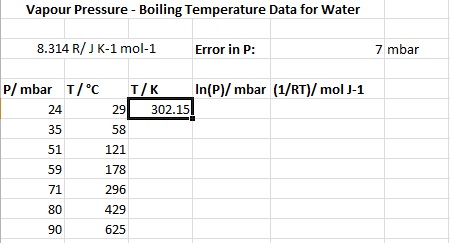
4.	Now press Enter. The formula will disappear and be replaced with the calculated value. Click on cell C6 again. Notice that the calculated value, not the formula, is displayed in the cell. The formula itself is shown in the box above the columns, next to the = sign. If you ever need to edit the cell formula, you can do so by clicking on the relevant part of the formula displayed in the formula box.
5.	We now need to repeat this calculation for the other temperature values. However, rather than typing the appropriate formula into every cell, we can get Excel to do this for us. Cell C6 on your worksheet should currently be bordered with a dark line, with a small dark square in the bottom right corner (see figure opposite). Move the cursor over this small square and press and hold the mouse button down.
6.	Move the mouse down, a box will appear around the block of cells that have been highlighted.
7.	Once the block of highlighted cells extends down to, and includes, C12 (see figure opposite) release the mouse button. Excel will automatically copy and paste the formula from C6 to the highlighted cells.
8.	Click on cell C7. Notice that the formula for this cell is =B7+273.15, i.e. Excel has automatically changed the cell/value used in the formula from b6 to b7. This will be true for the other cells as well.
9.	We now need to calculate the values for the remaining two columns. Select cell D6, type =ln(a6) and press Enter.	NOTE: =ln(a6) tells Excel to take the natural logarithm of the value in cell A6. Other useful mathematical functions are:   23 would be written in Excel as =2^3   4x105 would be written in Excel as =4E+05   e6 would be written in Excel as =exp(6) Obviously we could also replace the numbers in the examples above with a cell reference (e.g. =B6^2).
10.	Select cell E6, type =1/(a$3*c6) and press Enter.	NOTE: A $ has been included in the reference to the cell containing the gas constant (A3), since this tells Excel not to change the reference following the $ when the cell is copied. For example, if we had entered the formula as =1/(a3*c6) and had copied it to cell E7, the copied formula would read =1/(a4*c7), whereas copying the formula =1/(a$3*c6) will produce =1/(a$3*c7) in E7.
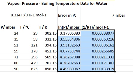
11.	Select cells D6 and E6 and repeat (for them) the block copy procedure outlined in steps 5-7. Your spreadsheet should now look like the figure opposite.