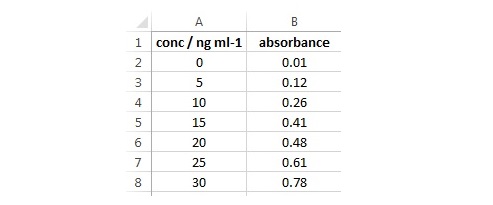
Using Excel 2013 - Adding Experimental Data
(VIEW THIS TUTORIAL AS A VIDEO)
|

|
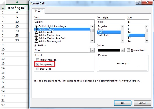
A Note on Superscripts & Subscripts
A better presentation of the title for the A column would be conc / ng ml-1. To do this: |

|
A Note on Keyboard Shortcuts
Many useful symbols can be entered using keyboard shortcuts. A few of these are detailed below:
| Alt + 0176 (on the numberpad) | to produce | ° |
| Alt + 0177 (on the numberpad) | to produce | ± |
| Alt + 0178 (on the numberpad) | to produce | ² |
| Alt + 0179 (on the numberpad) | to produce | ³ |
| Alt + 0181 (on the numberpad) | to produce | µ |
| Alt + 0188 (on the numberpad) | to produce | ¼ |
| Alt + 0189 (on the numberpad) | to produce | ½ |
| Alt + 0190 (on the numberpad) | to produce | ¾ |
| Alt + 0197 (on the numberpad) | to produce | Å |
| Alt + 0215 (on the numberpad) | to produce | × |
| Alt + 0247 (on the numberpad) | to produce | ÷ |
Greek symbols can be produced by changing the font to Symbol, and then typing the appropriate letter; e.g. a to produce a, D to produce D, etc.