Using Excel 2003 - 2.3) How to Format the Equation of a Trendline

Sometimes the trendline equation displayed on a graph will not be shown the number of decimal places or significant figures desired. In that situation the trendline equation will need to be reformatted as follows:

1. Click the mouse on the trendline equation until it is highlighted as shown below.
   
2. Right click the mouse over the trendline equation and select Format Data Labels... from the options displayed.
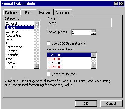
3. From the displayed Format Data Labels box, select the Number tab.
4. Select from the list under Category:, Number (if you wish to display the trendline equation to a defined number of decimal places) or Scientific (if you wish to display the trendline equation in scientific notation).
   
5. Specify the number of decimal places you wish to use in the box to the right of Decimal places: and click on OK.
   Example 1: If you selected Number and 1 Decimal places, then the equation in the example would be displayed as y = -4690.6x + 5.2
   Example 2: If you selected Scientific and 3 Decimal places, then the equation in the example would be displayed as y = -4.691E+03x + 5.223E+00