Using Excel 2003 - 2.2) How to Add Non-Linear Error Bars to a Graph
Sometimes the errors on a graph are not the same for every point. For example, if the pressure data used in Chapter 1.2 were assumed to have an error of ± 7 mbar, then the associated errors in a ln(P) vs 1/RT plot would not be the same size for every point (since a logarithm is a non-linear function).
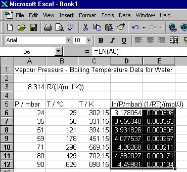
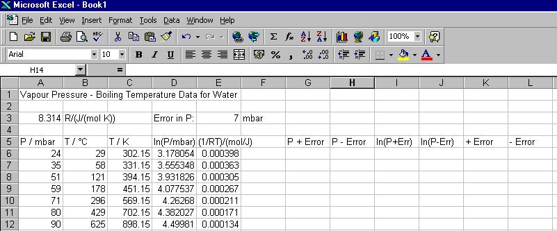
- Add column titles to your worksheet as shown in the figure below.
Note: To add the + Error and - Error titles you will need to enter in the cells '+ Error and '- Error. The ' tells Excel to display the entry as text.
- In columns G and H we will calculate values of the pressure plus its error and the pressure minus its error, i.e. the maximum and minimum possible pressures: Select cell G6 and type =A6+E$3 and then press [Enter]; Select cell H6 and type =A6-E$3 and then press [Enter].
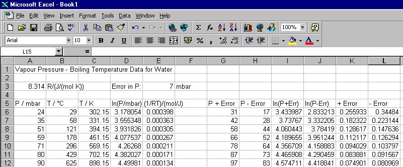
- In columns I and J we will will calculate the corresponding maximum and minimum values of ln(P): Select cell I6 and type =ln(g6) and then press [Enter]; Select cell J6 and type =ln(h6) and then press [Enter].
- Finally, in columns K and L we will calculate the positive and negative errors in ln(P), i.e. Positive Error in ln(P) = ln(P+Err)-ln(P) and Negative Error in ln(P) = ln(P)-ln(P-Err). This is done by entering the formulas =i6-d6 and =d6-j6 in cells K6 and L6.
- Block copy the new cells, so that data down to row 12 is generated, as shown in the figure below.
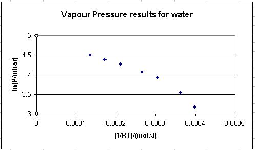
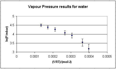
- Plot a graph of ln(P) versus 1/RT (as detailed in Chapter 1.4) and rescale it appropriately (as detailed in Chapter 2.1).
- Click the mouse on the Plot or Chart Area.
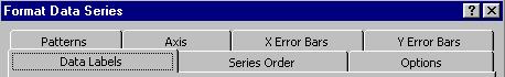
- Right click the mouse on one of the data points and select Format Data Series... from the options that appear.
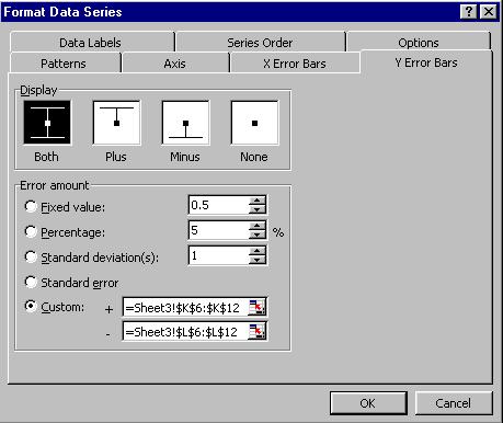
- The Format Data Series box will be displayed,click on the Y Error Bars tab.
- Click on Both under Display and make sure the option box to the left of Custom: is checked.
- Click on the box to the right of + and then block highlight the + Error cells in your workbook (K6 to K12). Click on the box to the right of - and then block highlight the - Error cells in your workbook (L6 to L12). The Format Data Series box should now look similar to that shown below.
- Click on OK. The graph will now include the non-linear error bars, as in the figure below.