Using Excel 2003 - 1.5) Adding a Trendline & Performing a Linear Regression

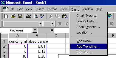
Using the data and graph generated in the first section of Chapter 1.4:

1. Select Chart, and then Add Trendline...
   
2. Click on the box above Linear.
   
3. Click on Options, and then on the white box to the left of Display equation on chart.
   
4. Click on OK.

Your spreadsheet should now look like the figure below.

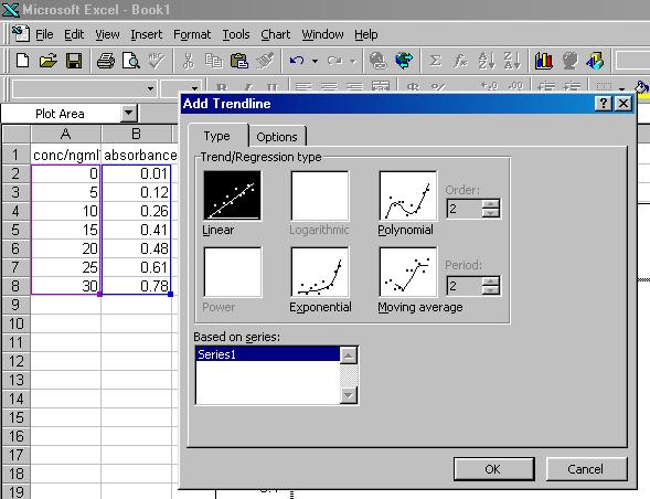
Note how the program has drawn a line of best fit through your data, and also plotted the equation of this straight line on the screen.

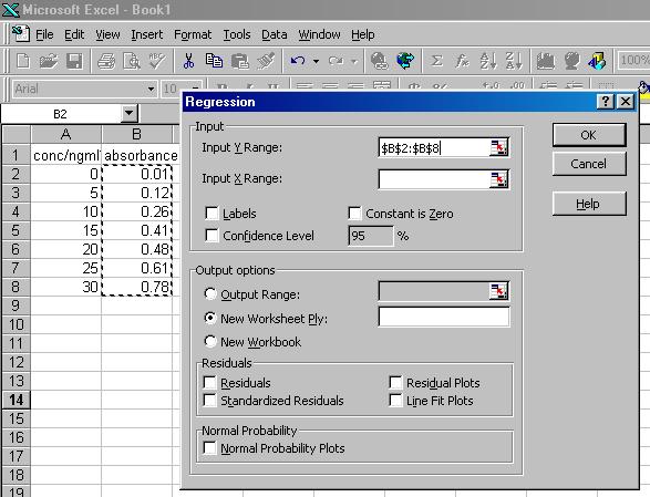
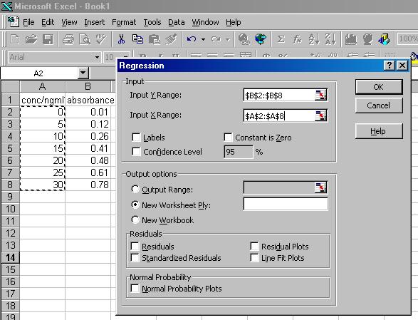
However, since our observations are affected by random errors and therefore have an associated statistical uncertainty, the gradient and y-intercept of our line of best fit also have errors. To calculate these errors use the following procedure:

1. Click on a cell over your data.
2. Under Tools, select Data Analysis...
   
3. Select Regression and then click on OK.
   
4. Make sure the cursor is flashing in the window to the right of Input Y Range.
   Enter the cell addresses for the data plotted along the y-axis by clicking and dragging down the relevant column (in this case B2 to B8).
   
5. Click in the window to the right of Input X Range.
   Enter the cell addresses for the data plotted along the x-axis by clicking and dragging down the relevant column (in this case A2 to A8).
   
6. Under Output options, click on the circle to the left of Output Range.
7. Make sure the flashing cursor is the window to the right of Output Range.
8. Click on the cell where you wish the output table to begin (in this case select A10). The cell address should appear in the window to the right of Output Range.
   
9. Makes sure the box to the left of Confidence Level has been ticked and then click on OK.

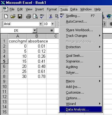
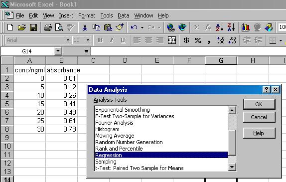
The data portion of your spreadsheet should now look like the figure below

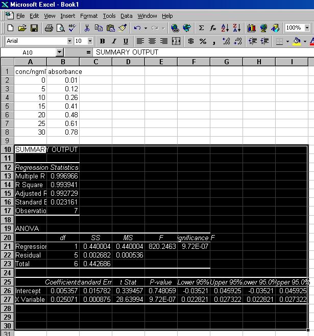
The SUMMARY OUTPUT details the formal statistics for the line of best fit. Most of the information given is beyond the scope of this course. However, you should pay attention to the values of the Coefficients, Lower 95% and Upper 95% values for the Intercept and X Variable (listed in the bottom table). The Coefficient of the Intercept corresponds to the value of the y-intercept of the line of best fit, and the Lower 95% and Upper 95% values for the Intercept are its 95% Confidence Limits, i.e. we are 95% sure the true value lies between these two limits. The Coefficient of the X Variable corresponds to the gradient of the line of best fit, and the Lower 95% and Upper 95% values for the X Variable are its 95% Confidence Limits.

For the data in this example we therefore have:

Gradient (G) = 0.0251
Upper95% - G = 0.0273 - 0.0251 = 0.0022; G - Lower95% = 0.0251 - 0.0228 = 0.0023
Therefore, G = 0.0251 ± 0.023

Intercept (I) = 0.00536
Upper95% - I = 0.04593 - 0.00536 = 0.04057; I - Lower95% = 0.00536 - (-0.03521) = 0.04057
Therefore, I = 0.005 ± 0.041